Optimizing SQL Server: Understanding Nested Loops, Hash Match, Merge Join, and Adaptive Join

In most database systems, join operations are essential for combining data from multiple tables. SQL Server, as a relational database engine, is built around efficiently joining tables to return relevant data. The execution plan in SQL Server reveals the specific join operators selected by the query optimizer to combine data.

When performing a join, SQL Server typically takes two data inputs, one from each table, and combines them based on the join criteria. The optimizer may select from one of four primary join operators:

• Nested Loops: This operator checks each row from the top dataset against every row from the bottom dataset to find matching values.
• Hash Match: In this method, a hash table is created using the top dataset, and the bottom dataset is then probed to find matching values.
• Merge Join: Both inputs are read simultaneously, and matching rows are merged based on the sorted join columns.
• Adaptive Join: Introduced in SQL Server 2017, this operator chooses either the Nested Loops or Hash Match method dynamically at runtime, based on the actual number of rows in the top dataset.

The choice of the join operator depends on the data’s size and how it is ordered, with each operator being optimal in different scenarios.

These operators implement several logical join types, including:

• Inner Join
• Outer Join (Left, Right, or Full)
• Semi Join (Left or Right)
• Anti Semi Join (Left or Right)
• Concatenation and Union

However, our focus here will be on the physical join operators, not the logical ones.

Understand the query

Let’s explore a query that retrieves employee data from the AdventureWorks2019 database. The query concatenates the FirstName and LastName columns to return the employee name in a more user-friendly format.

USE AdventureWorks2019
GO

SELECT e.JobTitle, a.City, p.LastName + ', ' + p.FirstName AS EmployeeName
 FROM HumanResources.Employee AS e
 INNER JOIN Person.BusinessEntityAddress AS bea
 ON e.BusinessEntityID = bea.BusinessEntityID
 INNER JOIN Person.Address AS a
 ON bea.AddressID = a.AddressID
 INNER JOIN Person.Person AS p
 ON e.BusinessEntityID = p.BusinessEntityID;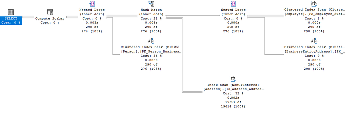

When analyzing the execution plan, it’s useful to understand its flow. You can either follow the arrows from right to left, or follow the operators as they appear in the query.

In our case, the query optimizer first uses a Nested Loops operator to join the Employee and BusinessEntityAddress tables, then applies a Hash Match to combine those rows with the Address table, and finally uses another Nested Loops operator to join the data with the Person table.

Let’s focus on how each join operator functions within this execution plan.

Nested Loops operator

The Nested Loops operator is a basic yet effective method for joining data. It operates by comparing each row from the outer input (top input) to each row from the inner input (bottom input). This method is particularly efficient when the outer input is small and searching the inner input is cheap, which is often achieved by indexing the join column of the inner table.

This operator is similar to a cursor in that it uses two cursors: one for the outer input data set, which is processed row by row, and another for the inner input, which is processed for each row of the outer input. Consequently, the operator or operators in the inner input will execute multiple times — once for each row in the outer input.

Nested Loops is highly efficient when the outer input is small and searching the inner input is inexpensive. This is often achieved through indexing the “inner table” on the join column, which is common in simple join operations.

This join method is particularly effective when the outer input has low cardinality and the inner input can be accessed with low cost per execution. When compared to other join operators, such as Merge Join (best for sorted data streams), Hash Match (ideal for large unsorted data sets), and Adaptive Join (used when both Nested Loops and Hash Match are viable but the optimizer defers the final decision until runtime), Nested Loops remains a strong contender for specific cases.

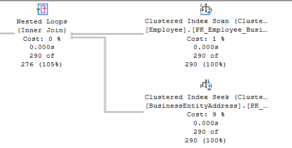
For example, in the current plan, the Employee table’s clustered index scan (the outer input) returns 290 rows. For each row, the Nested Loops operator then searches the BusinessEntityAddress table to find matching BusinessEntityID values. This search involves 290 index seek operations.

There are two ways that the Nested Loops operator can resolve a join condition.: Outer References and Predicate.

We’re not focus on this…but here we go!

Outer References (Dynamic Inner Input): In this approach, operators on the inner input rely on values from the outer input. If, for example, 10 values are passed from the outer input to the inner input (known as Outer References), the inner input is executed 10 times, searching for matching rows. The inner input will return only the matching rows, so the Nested Loops operator doesn’t need to do extra work to validate the matches.

Predicate (Static Inner Input): This method occurs when the inner input has no pushed-down values, meaning it always returns the same results during each execution. The Nested Loops operator applies the join predicate to the rows from the inner input and only returns matching rows.

Insight: Seek predicate inputs are generally less efficient than Outer References. The SQL Server optimizer usually opts for a static inner input when a dynamic one is not feasible or practical.

Extra Tips: Rebinds and Rewinds are only relevant when the Nested Loops operator interacts with one of the operators: Index Spool — Remote Query — Row Count Spool — Sort — Table Spool — Table valued function

Hash Match (join)

The Hash Match operator creates a hash table in memory from the top input (build input), then uses this hash table to probe the second input (probe input) to find matching rows.

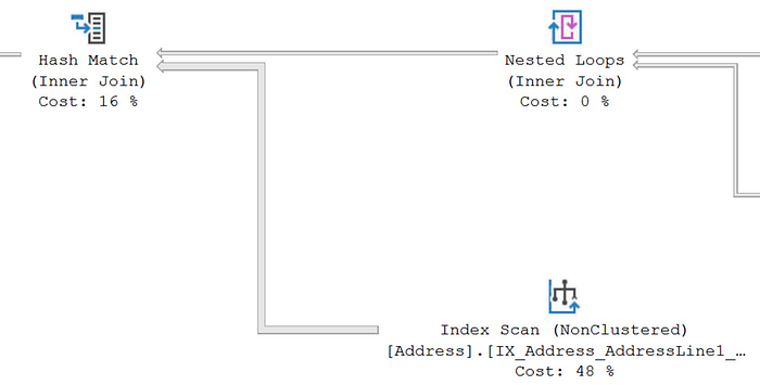
In this scenario, the Build input consists of the 290 rows from the Nested Loops operator, while the Probe input contains 19,614 rows resulting from a non-clustered index scan on the Address table. The Hash Match operator hashes the AddressID from the Build input and stores it in the hash table. It then compares each row from the Probe input, hashing the AddressID and checking if it matches the values in the hash table.

While the Hash Match operator is often used when data inputs are unsorted or large, it can be inefficient if the build input exceeds the optimizer’s memory grant, causing the data to spill to disk.

A hash table is a data structure in which SQL Server attempts to divide all the elements into equal-sized categories, or buckets, to allow quick access to the elements. The hashing function determines into which bucket an element goes. For example, SQL Server can take a column from a table, hash it into a hash value, and then store the matching rows in memory, within the hash table, in the appropriate bucket.

Attention

A Hash Match join operator is blocking during the Build phase. It has to gather all the data in order to build a hash table prior to performing its join operations and producing output. The optimizer will only tend to choose Hash Match joins in cases where the inputs are not sorted according to the join column. Hash Match joins can be efficient in cases where there are no usable indexes or where significant portions of the index will be scanned. If the inputs are already sorted on the join column, or are small and cheap to sort, then the optimizer may often opt to use a Merge Join instead.

However, a Hash Match join is often the best choice when you have two unsorted inputs, both large, or one small and one large. The optimizer will always choose what it estimates to be the smaller of the data inputs to be the Build input, which provides the values in the hash table. The goal is many hash buckets with few rows per bucket (i.e. minimal hash collisions,as few duplicate hashed values as possible). This makes finding matching rows in the Probe input fast, even with two large inputs, because the optimizer only needs to search for matches in the basket with the same hash value, instead of scanning all the rows.

Performance problems with Hash Match only really occur when the Build input is much larger than the optimizer anticipated, so that it exceeds the memory grant, and subsequently spills to disk.

Seeing a Hash Match join in an execution plan sometimes indicates:

• A missing or unusable index;
• A WHERE clause with a calculation or conversion that makes it nonSARGable (a commonly used term meaning that the search argument, “sarg,” can’t be used) — this means it won’t use an existing index.

So and about Merge Join?

A Merge Join operator operates exclusively on ordered data. It takes two inputs and utilizes the fact that both inputs are sorted on the join column, allowing it to simply merge the two datasets by matching corresponding values. This process is highly efficient because the order of the values in both inputs is already aligned. Additionally, a Merge Join is a non-blocking operator, meaning it doesn’t need to hold up processing while joining rows, resulting in better performance as it passes each matched row to the next operator.

When both data inputs are pre-sorted by the join column, the Merge Join becomes one of the most efficient join operations. However, if the data isn’t ordered, the optimizer must add a Sort operator to arrange the data for the join, which can negatively impact performance. Sorting adds extra overhead, making plans with a Merge Join less efficient, depending on how the sorting is handled.

On the other hand, since a Merge Join guarantees that the result of the join will be ordered, it might sometimes be worth accepting the cost of a single Sort operation to ensure that the output is correctly ordered. This is especially useful when subsequent Merge Joins in the execution plan can benefit from the ordered result.

Let’s work

Use AdventureWorks2019
GO

SELECT c.CustomerID
FROM Sales.SalesOrderDetail AS sod
 INNER JOIN Sales.SalesOrderHeader AS soh
 ON sod.SalesOrderID = soh.SalesOrderID
 INNER JOIN Sales.Customer AS c
 ON soh.CustomerID = c.CustomerID;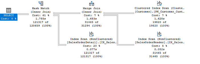

The optimizer has chosen a Merge Join operator to perform the INNER JOIN between the Customer and SalesOrderHeader tables, matching values based on the CustomerID. Since the query doesn’t include a WHERE clause, a scan is performed on both tables to retrieve all rows. It’s important to note that the optimizer may rearrange the order of tables in the execution plan, which might not reflect the exact order written in the query. The optimizer selects the Customer table, which has guaranteed unique values, as the top input, resulting in a one-to-many join.

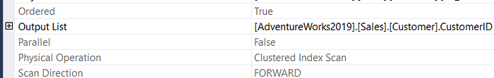
The data from the top input, a Clustered Index Scan on the Customer table, is already sorted by CustomerID. The bottom input comes from a Nonclustered Index Scan on the SalesOrderHeader table. Both inputs are sorted by the join column, as confirmed in the properties of the Merge Join operator.

The key to Merge Join performance lies in the sorting of the input data by the join columns. We can verify this by checking the properties of the operators, which indicate that both scan results are already ordered. This sorting ensures that the Merge Join can efficiently match rows between the two tables without additional sorting, making it a highly efficient join method when the data is appropriately ordered.

The output of the scans is ordered by the join columns, and no additional sorting is necessary. If one or more of the inputs is not ordered, and the query optimizer chooses to sort the data in a separate operation before it performs a Merge Join, it might indicate that you need to reconsider your indexing strategy, especially if the Sort operation is for a large data input.

Last one: Adaptive Join

Introduced in SQL Server 2017, and also available in Azure SQL Database and Azure SQL Data Warehouse, the Adaptive Join is a new join operation. The optimizer can choose an Adaptive Join operator to defer the exact choice of physical join algorithm, either a Hash Match or a Nested Loops, until runtime, when the actual number of rows in the top input is known rather than estimated.

To see the Adaptive Join in action, we need a batch mode plan, which requires a column store index.

DROP INDEX IF EXISTS ix_csTest ON Production.TransactionHistory;
GO
CREATE NONCLUSTERED COLUMNSTORE INDEX IX_CSTest
ON Production.TransactionHistory
(
 TransactionID,
 ProductID,
 ActualCost
);


SELECT p.Name AS ProductName,
 th.ActualCost
FROM Production.TransactionHistory AS th
 JOIN Production.Product AS p
 ON p.ProductID = th.ProductID
WHERE th.ActualCost > 0
 AND th.ActualCost < .21;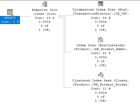

As you can observe, the Adaptive Join uses three inputs instead of the usual two. The top input is a scan of a nonclustered columnstore index, while the lower inputs include an Index Scan and a Clustered Index Seek, which support either a Hash Match or Nested Loops join.

Similar to the Hash Match join operator, the Adaptive Join has a “Build” phase where it stores the rows from the top input in a hash table in memory, requiring a memory grant. This phase is blocking, meaning the operator needs to gather all the data before proceeding.

Once the top input is processed and stored in the hash table, the exact number of rows is determined. This row count is then used to decide whether to proceed with a Hash Match or a Nested Loops join. The decision is based on comparing the number of rows in the hash table to a threshold value set by the optimizer, which can vary depending on the data structure, the query, and index statistics (you can see this value in the properties of the Adaptive Join operator).

If the number of rows exceeds the threshold, the optimizer chooses the Hash Match join. The hash table will use the upper input to gather the necessary data, and the operation proceeds as a typical Hash Match. For example, an Index Scan against the Product table using the AK_Product_Name index may be performed. If the number of rows is below the threshold, the optimizer switches to the Nested Loops method, performing a Clustered Index Seek on the Product table using a different index, PK_Product_ProductID, for each row in the hash table.

The Adaptive Join essentially gives the optimizer the flexibility to choose the most efficient join method based on the actual row count. For low row counts, the Nested Loops branch will execute, which may cost slightly more than directly using Nested Loops, but it avoids the inefficiency of a Hash Match when dealing with small data sets. For high row counts, the plan will behave similarly to a standard Hash Match join, resulting in an optimal execution plan.

Conclusion

In conclusion, SQL Server provides a variety of physical join operators, each suited to different types of data sets and query scenarios. Understanding the behavior and performance characteristics of these join operators — Nested Loops, Hash Match, Merge Join, and Adaptive Join — is essential for optimizing query performance. Each operator has its strengths depending on the structure and size of the data being joined, as well as the presence of indexes or sorting.

• Nested Loops is efficient when dealing with small data sets or indexed columns, making it a great choice for simple, fast joins.
• Hash Match works well with large, unsorted data sets and is often used when the inputs are not indexed or sorted on the join column.
• Merge Join excels when data is pre-sorted or indexed on the join column, allowing for efficient and fast merging of the two data streams.
• Adaptive Join, introduced in SQL Server 2017, dynamically switches between Nested Loops and Hash Match during query execution, offering flexibility based on the actual row count, thus optimizing performance in variable data conditions.

By examining the execution plan and understanding how each join operator works, you can identify opportunities to fine-tune your queries, improve indexing strategies, and ensure your database performs at its best. Ultimately, SQL Server’s optimizer makes intelligent decisions to balance speed and efficiency, but understanding how it works enables you to better guide and enhance those decisions.

Source Reference: SQL Server Execution Plans By Grant Fritchey — Third Edition Book